It is good practice to provide a way to drain entrapped condensate from the pressure lines, it’s mandatory to entrap condensate before that reach pressure sensor, refer to the below figure as a possible arrangement. The proposed arrangement mimic a five ways manifold, that is commonly used in industrial and scientific applications, use of a manifold can be unpractical on standard sized models anyway consider the presented scheme as conceptual to expose typical operation scenery.

Since the scheme is conceptual the valves in the real world can be simply replaced by plugs and pressure line interruptions. D1 and D2 represent the drain valves, locate this valves at a piezometric head below the ADC, the eventually present condensate will fill the drain lines. To ease the drain circulation consider to maintain never less than 3° of inclination of pressure lines.

During pitot operation maybe some port can become clogged, sometimes it’s unavoidable to blow air from the pressure line into the probe, in this situation the priority is to don’t damage ADC sensors.

Pneumatic transmission lag

It takes some time for the pressure to propagate from the input ports to the sensors,  that’s the transmission lag. Basic knowledge of this phenomenon can help to define some performance limits. As general rule consider to maintain pressure lines as short as you can to limit pressure transmission lag[4] [pag 5][6][2] [Fig.19] and maximize dynamic response, if possible keep you pressure lines always side by side so they will be maintained at the same temperature and will have the same length; this last point ensure that the pressure is even along both the lines, no internal differential pressure buildup due to temperature differences.  Pressure line material should be able to resist to condensate exposure and ensure that the lines will not deform during operations. Regarding dynamic behavior [1] [Pag 22] if the lag is extremely reduced the readings may be affected by noise due to the high bandwidth of the transmission line; that are very sensible problems, it’s not sufficient to reduce the lag but it’s also needed some degree of pressure damping. Numeric example, data from the Pitot we will present as example realization ahead in the page. According to [7] [7 pag 5] and using the following data from our pitot,

For preliminary evaluation, it can be used the Eq.3 for the asymptotic case[7] [Pag 9] that lead to a resonance frequency value of 133 Hz. Refer to the following figure 3 to visualize the frequency response of our pressure line, this figure was calculated with the Equation 2 at page 9 [7]

You can play around with the parameters downloading this scilab file. From the figure you can observe the resonance peak, the response of the system is unitary up to 15Hz so under this frequency the pressure transfer from the port to the sensor is ideal. Reference [7] conclusions will clarify many interesting design aspects and since the model is validated with real world data it’s possible to use the transfer function to compensate higher frequency readings. Ability to predict dynamic performance is fundamental when using more complex devices, as rotating probe designs, or in the loop operation of the sensor.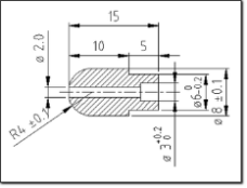

Figure 4 – Hemispherical Pitot head

Angle of attack and sideslip When the probe is not perfectly lined with the relative wind it will perform not optimally. If the measure the AOA or AOS is unavailable the only approach is to choice a probe that work well at different angles, anyway in the classical pitot range there are no probes able to cope with 20°off center angles without abruptly changing the coefficient of calibration so the most precise measurements will be at low angles. Have a look at coefficients deviation vs the angle in[5] [Fig. 36]. When information about flight AOA and AOS is available a real-time compensation on the airspeed measurements can be practically usable.

Design example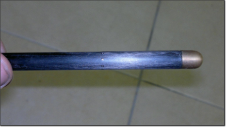

Figure 5 – Realized Pitot Head, Carbon Fiber and brass

Our design will be quite simple. First of all, we need a source for the calibration parameter and off angle probe behavior data. Excluding the use of a wind tunnel and books, there is some others source of information. For example, but not only NACA, NASA, NPL and also from AFNOR 10-112 and other industrial design codes. Formally at least one point calibration is needed because almost every published data refer to a single pitot and not to a production batch with well-defined machining tolerances and doing so it’s possible to correct installation position errors. By experience, if is not sought an extreme instruments performance and the probe is mounted in front of the aircraft the coefficients from bibliography can be directly used, accounting simply for an extended uncertainty. For sake of simplicity and free online availability of documentation, our design will be based on[5]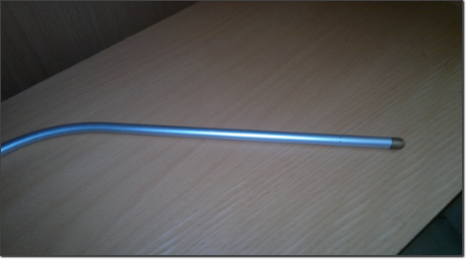

Figure 7 – Aluminum alloy detail

Because our speed formula is:

So from[5] pag. 5-6 it’s possible to define  According to [5][1] pag 5-6 the term E of error is neglected as we will operate the probe at a sufficient high Reynolds number, the terms depending on Mach number should be accounted so the formula simplifies to .

In many practical cases, this term contribution can be safely neglected as it is of small magnitude.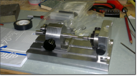

Figure 8 – DIY Dead center, drill

In [5] [1 appendix figures] you find beautiful laboratory images of the boundary layer for different pitots at different speeds/Reynolds number. Looking for a simply realizable pitot and with a calibration factor near to 1 HNG[5][Par. 26.6 ]is chosen. The tip of this pitot is a hemisphere, the external dimension D is 5/16” or 7.94mm, the static pressure ports are located at 4.5D from the tip and consist of one annulus of 8 holes of diameter 1.01 mm, total pressure hole is 1.84 mm[5] [Fig.1]. Measures are weird in mm as they are derived from imperial system, anyway, I rounded the measures to ease the machining phase. Modification of dimensions can lead to modifying the probe characteristics, eventually, that will be checked/compensated during the calibration phase.

You find the drawing of the head on Figure 4, you can get the complete drawing in PDF or you can download also a scale CAD drawing here.